Ana María Tárano

🗺️ I advance human-centered geospatial machine learning to support decision-making for food security and environmental resilience.
🤝 My research practice is emergent from a design thinking ethos.
HOME | BIO-SKETCH | RECENT PROJECTS | EDUCATION | PREVIOUS WORK | PUBLICATIONS | RECENT PRESENTATIONS | AWARDS
Get started with open reproducible science! (API version)

It’s another ESIIL Earth Data Science Workflow
This notebook contains your next environmental data science (EDS) coding challenge! Before we get started, make sure to read or review the guidelines below. These will help make sure that your code is readable and reproducible.
Don’t get caught by these interactive coding notebook gotchas
Image source: https://alaskausfws.medium.com/whats-big-and-brown-and-loves-salmon-e1803579ee36
These are the most common issues that will keep you from getting started and delay your code review:
Run your code in the right environment to avoid import errors
We’ve created a coding environment for you to use that already has all the software and libraries you will need! When you try to run some code, you may be prompted to select a kernel. The kernel refers to the version of Python you are using. You should use the base kernel, which should be the default option.
Always run your code start to finish before submitting
Before you commit your work, make sure it runs reproducibly by clicking:
Restart(this button won’t appear until you’ve run some code), thenRun All
Check your code to make sure it’s clean and easy to read
-
Format all cells prior to submitting (right click on your code).
-
Use expressive names for variables so you or the reader knows what they are.
-
Use comments to explain your code – e.g.
# This is a comment, it starts with a hash sign
Label and describe your plots
Make sure each plot has: * A title that explains where and when the data are from * x- and y- axis labels with units where appropriate * A legend where appropriate
Get started with open reproducible science!
Open reproducible science makes scientific methods, data and outcomes available to everyone. That means that everyone who wants should be able to find, read, understand, and run your workflows for themselves.
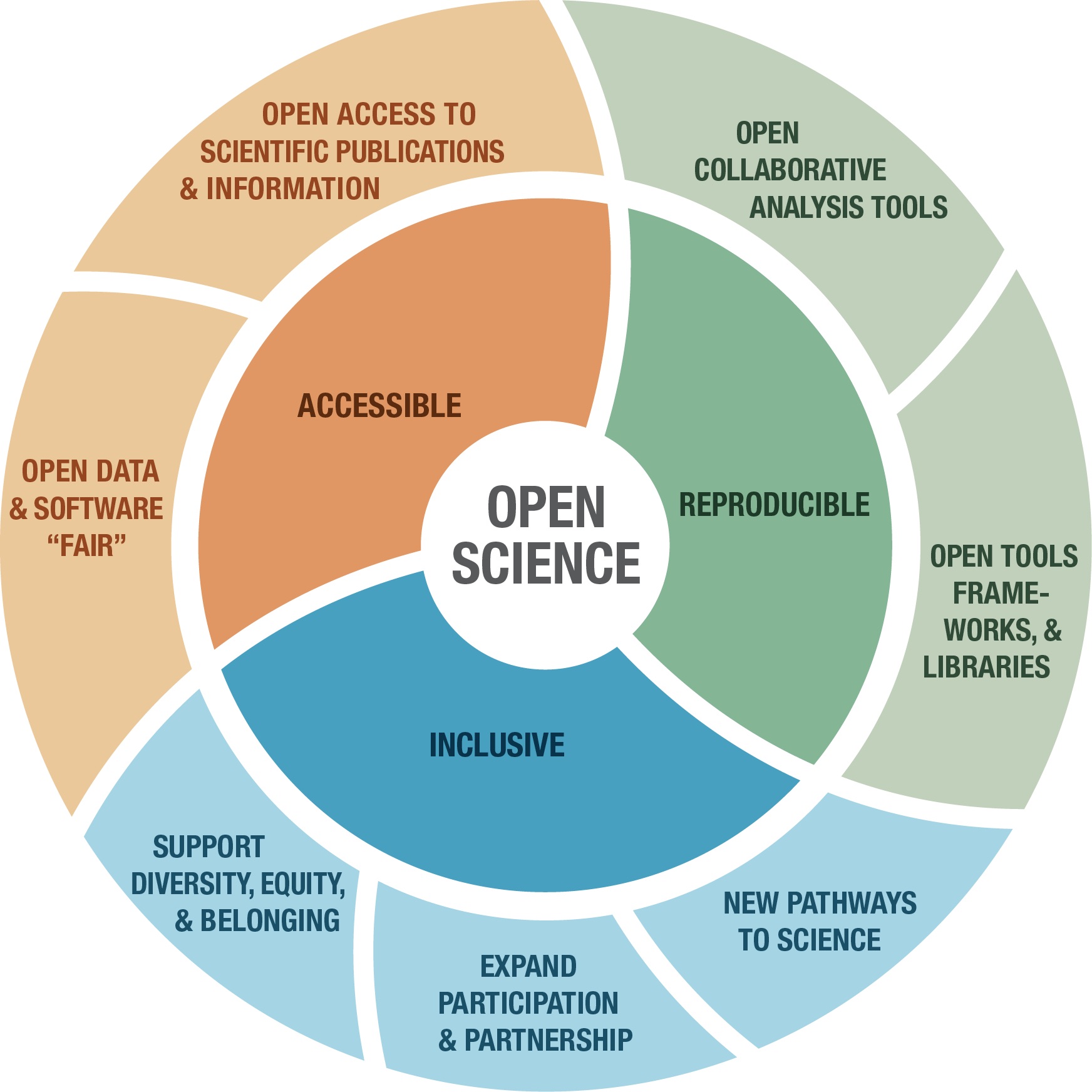
Image from https://www.earthdata.nasa.gov/esds/open-science/oss-for-eso-workshops
Few if any science projects are 100% open and reproducible (yet!). However, members of the open science community have developed open source tools and practices that can help you move toward that goal. You will learn about many of those tools in the Intro to Earth Data Science textbook. Don’t worry about learning all the tools at once – we’ve picked a few for you to get started with.
Further reading
What does open reproducible science mean to you?
Create a new Markdown cell below this one using the
+ Markdownbutton in the upper left.In the new cell, answer the following questions using a numbered list in Markdown:
- In 1-2 sentences, define open reproducible science.
- In 1-2 sentences, choose one of the open source tools that you have learned about (i.e. Shell, Git/GitHub, Jupyter Notebook, Python) and explain how it supports open reproducible science.
- Open reproducible science is a scientific philosophy that makes data, methods, and code accessible to most (assumes level of access to computational resources, reliable internet, and background knowledge) by removing barriers to reproduce scientific results.
- Git supports open reproducible science by enabling code, data (through APIs or urls), and results to be ran, edited, and evaluated in a public space by many.
Human-readable and Machine-readable
Create a new Markdown cell below this one using the ESC + b keyboard shortcut.
In the new cell, answer the following question in a Markdown quote:
- In 1-2 sentences, does this Jupyter Notebook file have a machine-readable name? Explain your answer.
The exclamation point and spaces make this file not machine-readable.
Readable, well-documented scientific workflows are easier to reproduce
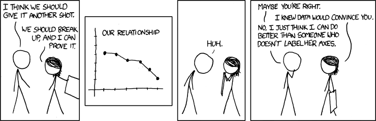
As the comic below suggests, code that is hard to read is also hard to get working. We refer to code that is easy to read as clean code.
)](https://imgs.xkcd.com/comics/wanna_see_the_code.png)
In the prompt below, list 3 things you can do to write clean code, and then list 3 more advantages of doing so.
- Edit the text below. You may have to double click.
- You can use examples from the textbook, or come up with your own.
- Use Markdown to format your list.
I can write clean code by: breaking up code using different cells, using markdown cells to introduce those conding cells, and save variables with their descriptive name
Advantages of clean code include: being able to remember quickly what you did and have others understand your code quickly
What the fork?! Who wrote this?
Below is a scientific Python workflow. But something’s wrong – The code won’t run! Your task is to follow the instructions below to clean and debug the Python code below so that it runs.
Tip
Don’t worry if you can’t solve every bug right away. We’ll get there! The most important thing is to identify problems with the code and write high-quality GitHub Issues
At the end, you’ll repeat the workflow for a location and measurement of your choosing.
Alright! Let’s clean up this code. First things first…
Machine-readable file names
Rename this notebook if necessary with an expressive and machine-readable file name
Python packages let you use code written by experts around the world
Because Python is open source, lots of different people and organizations can contribute (including you!). Many contributions are in the form of packages which do not come with a standard Python download.
Read more
In the cell below, someone was trying to import the pandas package, which helps us to work with tabular data such as comma-separated value or csv files.
Your task
- Correct the typo below to properly import the pandas package under its alias pd.
- Run the cell to import pandas
# Import pandas
import pandas as pd
Once you have run the cell above and imported pandas, run the cell
below. It is a test cell that will tell you if you completed the task
successfully. If a test cell isn’t working the way you expect, check
that you ran your code immediately before running the test.
# DO NOT MODIFY THIS TEST CELL
points = 0
try:
    pd.DataFrame()
    points += 5
    print('\u2705 Great work! You correctly imported the pandas library.')
except:
    print('\u274C Oops - pandas was not imported correctly.')
print('You earned {} of 5 points for importing pandas'.format(points))
✅ Great work! You correctly imported the pandas library.
You earned 5 of 5 points for importing pandas
There are more Earth Observation data online than any one person could ever look at
NASA’s Earth Observing System Data and Information System (EOSDIS) alone manages over 9PB of data. 1 PB is roughly 100 times the entire Library of Congress (a good approximation of all the books available in the US). It’s all available to you once you learn how to download what you want.
Here we’re using the NOAA National Centers for Environmental Information (NCEI) Access Data Service application progamming interface (API) to request data from their web servers. We will be using data collected as part of the Global Historical Climatology Network daily (GHCNd) from their Climate Data Online library program at NOAA.
For this example we’re requesting daily summary data in Boulder, CO (station ID USC00050848) located on the NOAA Campus (39.99282°, -105.26683°).
Your task:
- Research the Global Historical Climatology Network - Daily data source.
- In the cell below, write a 2-3 sentence description of the data source. You should describe:
- who takes the data
- where the data were taken
- what the maximum temperature units are
- how the data are collected
- Include a citation of the data (HINT: See the ‘Data Citation’ tab on the GHCNd overview page).
YOUR DATA DESCRIPTION AND CITATION HERE 🛎️
TODO
You can access NCEI GHCNd Data from the internet using its API 🖥️ 📡 🖥️
The cell below contains the URL for the data you will use in this part of the notebook. We created this URL by generating what is called an API endpoint using the NCEI API documentation.
Note
An application programming interface (API) is a way for two or more computer programs or components to communicate with each other. It is a type of software interface, offering a service to other pieces of software (Wikipedia).
However, we still have a problem - we can’t get the URL back later on because it isn’t saved in a variable. In other words, we need to give the url a name so that we can request in from Python later (sadly, Python has no ‘hey what was that thingy I typed yesterday?’ function).
Read more
Check out the textbook section on variables
Your task
Pick an expressive variable name for the URL
HINT: click on the
Variablesbutton up top to see all your variables. Your new url variable will not be there until you define it and run the codeReformat the URL so that it adheres to the 79-character PEP-8 line limit
HINT: You should see two vertical lines in each cell - don’t let your code go past the second line
At the end of the cell where you define your url variable, call your variable (type out its name) so it can be tested.
boulder_url = ('https://www.ncei.noaa.gov/access/services/data/v1?'
               'dataset=daily-summaries&'
               'dataTypes=TOBS,PRCP&'
               'stations=USC00050848&'
               'startDate=1893-10-01&'
               'endDate=2024-02-18&'
               'includeStationName=true&'
               'includeStationLocation=1&'
               'units=standard')
boulder_url
'https://www.ncei.noaa.gov/access/services/data/v1?dataset=daily-summaries&dataTypes=TOBS,PRCP&stations=USC00050848&startDate=1893-10-01&endDate=2024-02-18&includeStationName=true&includeStationLocation=1&units=standard'
# DO NOT MODIFY THIS TEST CELL
resp_url = _
points = 0

if type(resp_url)==str:
    points += 3
    print('\u2705 Great work! You correctly called your url variable.')
else:
    print('\u274C Oops - your url variable was not called correctly.')

if len(resp_url)==218:
    points += 3
    print('\u2705 Great work! Your url is the correct length.')
else:
    print('\u274C Oops - your url variable is not the correct length.')

print('You earned {} of 6 points for defining a url variable'.format(points))
✅ Great work! You correctly called your url variable.
✅ Great work! Your url is the correct length.
You earned 6 of 6 points for defining a url variable
Download and get started working with NCEI data
The pandas library you imported can download data from the internet
directly into a type of Python object called a DataFrame. In the
code cell below, you can see an attempt to do just this. But there are
some problems…
You’re ready to fix some code!
Your task is to:
Leave a space between the
#and text in the comment and try making the comment more informativeMake any changes needed to get this code to run. HINT: The
my_urlvariable doesn’t exist - you need to replace it with the variable name you chose.Modify the
.read_csv()statement to include the following parameters:
index_col='DATE'– this sets theDATEcolumn as the index. Needed for subsetting and resampling later onparse_dates=True– this letspythonknow that you are working with time-series data, and values in the indexed column are date time objectsna_values=['NaN']– this letspythonknow how to handle missing valuesClean up the code by using expressive variable names, expressive column names, PEP-8 compliant code, and descriptive comments
Make sure to call your DataFrame by typing it’s name as the last
line of your code cell Then, you will be able to run the test cell
below and find out if your answer is correct.
# Read daily summaries from Boulder
# Columns include: "DATE", "STATION", "NAME", "LATITUDE", "LONGITUDE",
# "ELEVATION", "PRCP", AND "TOBS"
boulder_df = pd.read_csv(
  boulder_url,
  index_col='DATE',
  parse_dates = True,
  na_values = ['NaN'])
boulder_df
| STATION | NAME | LATITUDE | LONGITUDE | ELEVATION | PRCP | TOBS | |
|---|---|---|---|---|---|---|---|
| DATE | |||||||
| 1893-10-01 | USC00050848 | BOULDER, CO US | 39.99282 | -105.26683 | 1673.0 | 0.94 | NaN |
| 1893-10-02 | USC00050848 | BOULDER, CO US | 39.99282 | -105.26683 | 1673.0 | 0.00 | NaN |
| 1893-10-03 | USC00050848 | BOULDER, CO US | 39.99282 | -105.26683 | 1673.0 | 0.00 | NaN |
| 1893-10-04 | USC00050848 | BOULDER, CO US | 39.99282 | -105.26683 | 1673.0 | 0.04 | NaN |
| 1893-10-05 | USC00050848 | BOULDER, CO US | 39.99282 | -105.26683 | 1673.0 | 0.00 | NaN |
| ... | ... | ... | ... | ... | ... | ... | ... |
| 2024-02-14 | USC00050848 | BOULDER, CO US | 39.99282 | -105.26683 | 1673.0 | 0.00 | 41.0 |
| 2024-02-15 | USC00050848 | BOULDER, CO US | 39.99282 | -105.26683 | 1673.0 | 0.00 | 39.0 |
| 2024-02-16 | USC00050848 | BOULDER, CO US | 39.99282 | -105.26683 | 1673.0 | 0.20 | 23.0 |
| 2024-02-17 | USC00050848 | BOULDER, CO US | 39.99282 | -105.26683 | 1673.0 | 0.22 | 23.0 |
| 2024-02-18 | USC00050848 | BOULDER, CO US | 39.99282 | -105.26683 | 1673.0 | 0.00 | 42.0 |
46112 rows × 7 columns
# DO NOT MODIFY THIS TEST CELL
tmax_df_resp = _
points = 0

if isinstance(tmax_df_resp, pd.DataFrame):
    points += 1
    print('\u2705 Great work! You called a DataFrame.')
else:
    print('\u274C Oops - make sure to call your DataFrame for testing.')

print('You earned {} of 2 points for downloading data'.format(points))
✅ Great work! You called a DataFrame.
You earned 1 of 2 points for downloading data
HINT: Check out the
type()function below - you can use it to check that your data is now inDataFrametype object
# Check that the data was imported into a pandas DataFrame
type(boulder_df)
pandas.core.frame.DataFrame
Clean up your DataFrame
Use double brackets to only select the columns you want in your DataFrame
Make sure to call your DataFrame by typing it’s name as the last
line of your code cell Then, you will be able to run the test cell
below and find out if your answer is correct.
boulder_df = boulder_df[['PRCP', 'TOBS']]
boulder_df
| PRCP | TOBS | |
|---|---|---|
| DATE | ||
| 1893-10-01 | 0.94 | NaN |
| 1893-10-02 | 0.00 | NaN |
| 1893-10-03 | 0.00 | NaN |
| 1893-10-04 | 0.04 | NaN |
| 1893-10-05 | 0.00 | NaN |
| ... | ... | ... |
| 2024-02-14 | 0.00 | 41.0 |
| 2024-02-15 | 0.00 | 39.0 |
| 2024-02-16 | 0.20 | 23.0 |
| 2024-02-17 | 0.22 | 23.0 |
| 2024-02-18 | 0.00 | 42.0 |
46112 rows × 2 columns
# DO NOT MODIFY THIS TEST CELL
tmax_df_resp = _
points = 0

summary = [round(val, 2) for val in tmax_df_resp.mean().values]
if summary == [0.05, 54.53]:
    points += 4
    print('\u2705 Great work! You correctly downloaded data.')
else:
    print('\u274C Oops - your data are not correct.')
print('You earned {} of 5 points for downloading data'.format(points))
✅ Great work! You correctly downloaded data.
You earned 4 of 5 points for downloading data
Plot the precpitation column (PRCP) vs time to explore the data
Plotting in Python is easy, but not quite this easy:
boulder_df.plot()
<Axes: xlabel='DATE'>
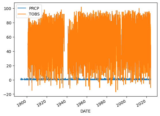
You’ll always need to add some instructions on labels and how you want your plot to look.
Your task:
- Change
dataframeto yourDataFramename.- Change
y=to the name of your observed temperature column name.- Use the
title,ylabel, andxlabelparameters to add key text to your plot.- Adjust the size of your figure using
figsize=(x,y)wherexis figure width andyis figure heightHINT: labels have to be a type in Python called a string. You can make a string by putting quotes around your label, just like the column names in the sample code (eg
y='TOBS').
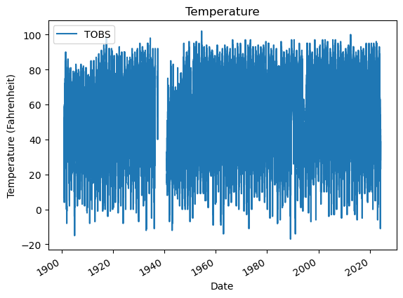
# Plot the data using .plot
boulder_df.plot(
    y='TOBS',
    title='Temperature',
    xlabel='Date',
    ylabel='Temperature (Fahrenheit)')
<Axes: title={'center': 'Temperature'}, xlabel='Date', ylabel='Temperature (Fahrenheit)'>
Want an EXTRA CHALLENGE?
There are many other things you can do to customize your plot. Take a look at the pandas plotting galleries and the documentation of plot to see if there’s other changes you want to make to your plot. Some possibilities include:
- Remove the legend since there’s only one data series
- Increase the figure size
- Increase the font size
- Change the colors
- Use a bar graph instead (usually we use lines for time series, but since this is annual it could go either way)
- Add a trend line
Not sure how to do any of these? Try searching the internet, or asking an AI!
Convert units
Modify the code below to add a column that includes temperature in Celsius. The code below was written by your colleague. Can you fix this so that it correctly calculates temperature in Celsius and adds a new column?
# Convert to celcius
boulder_df.loc[:, 'TCel'] = (boulder_df['TOBS'] - 32) * 5 / 9
boulder_df
| PRCP | TOBS | TCel | |
|---|---|---|---|
| DATE | |||
| 1893-10-01 | 0.94 | NaN | NaN |
| 1893-10-02 | 0.00 | NaN | NaN |
| 1893-10-03 | 0.00 | NaN | NaN |
| 1893-10-04 | 0.04 | NaN | NaN |
| 1893-10-05 | 0.00 | NaN | NaN |
| ... | ... | ... | ... |
| 2024-02-14 | 0.00 | 41.0 | 5.000000 |
| 2024-02-15 | 0.00 | 39.0 | 3.888889 |
| 2024-02-16 | 0.20 | 23.0 | -5.000000 |
| 2024-02-17 | 0.22 | 23.0 | -5.000000 |
| 2024-02-18 | 0.00 | 42.0 | 5.555556 |
46112 rows × 3 columns
# DO NOT MODIFY THIS TEST CELL
tmax_df_resp = _
points = 0

if isinstance(tmax_df_resp, pd.DataFrame):
    points += 1
    print('\u2705 Great work! You called a DataFrame.')
else:
    print('\u274C Oops - make sure to call your DataFrame for testing.')

summary = [round(val, 2) for val in tmax_df_resp.mean().values]
if summary == [0.05, 54.53, 12.52]:
    points += 4
    print('\u2705 Great work! You correctly converted to Celcius.')
else:
    print('\u274C Oops - your data are not correct.')
print('You earned {} of 5 points for converting to Celcius'.format(points))
✅ Great work! You called a DataFrame.
✅ Great work! You correctly converted to Celcius.
You earned 5 of 5 points for converting to Celcius
Want an EXTRA CHALLENGE?
- As you did above, rewrite the code to be more expressive
- Using the code below as a framework, write and apply a function that converts to Celcius. > Functions let you reuse code you have already written
- You should also rewrite this function and parameter names to be more expressive.
def convert_far2cel(temp_farenheit):
    """Convert temperature to Celcius"""
    temp_celcius = (temp_farenheit- 32) * 5 / 9
    return temp_celcius # Put your equation in here

boulder_df['TOBS_Celcius'] = boulder_df['TOBS'].apply(convert_far2cel)
boulder_df['TOBS_Celcius']
/tmp/ipykernel_34028/4222664237.py:6: SettingWithCopyWarning:
A value is trying to be set on a copy of a slice from a DataFrame.
Try using .loc[row_indexer,col_indexer] = value instead

See the caveats in the documentation: https://pandas.pydata.org/pandas-docs/stable/user_guide/indexing.html#returning-a-view-versus-a-copy
  boulder_df['TOBS_Celcius'] = boulder_df['TOBS'].apply(convert_far2cel)


DATE
1893-10-01         NaN
1893-10-02         NaN
1893-10-03         NaN
1893-10-04         NaN
1893-10-05         NaN
                ...
2024-02-14    5.000000
2024-02-15    3.888889
2024-02-16   -5.000000
2024-02-17   -5.000000
2024-02-18    5.555556
Name: TOBS_Celcius, Length: 46112, dtype: float64
Subsetting and Resampling
Often when working with time-series data you may want to focus on a shorter window of time, or look at weekly, monthly, or annual summaries to help make the analysis more manageable.
Read more
Read more about subsetting and resampling time-series data in our Learning Portal.
For this demonstration, we will look at the last 40 years worth of data and resample to explore a summary from each year that data were recorded.
Your task
- Replace
start-yearandend-yearwith 1983 and 2023- Replace
dataframewith the name of your data- Replace
new_dataframewith something more expressive- Call your new variable
- Run the cell
# Subset the data
climate_1983_2023 = boulder_df.loc['1983':'2023'][['PRCP', 'TOBS', 'TOBS_Celcius']]
climate_1983_2023
| PRCP | TOBS | TOBS_Celcius | |
|---|---|---|---|
| DATE | |||
| 1983-01-01 | 0.0 | NaN | NaN |
| 1983-01-02 | 0.0 | NaN | NaN |
| 1983-01-03 | 0.0 | NaN | NaN |
| 1983-01-04 | 0.0 | NaN | NaN |
| 1983-01-05 | 0.0 | NaN | NaN |
| ... | ... | ... | ... |
| 2023-12-27 | 0.0 | 41.0 | 5.000000 |
| 2023-12-28 | 0.0 | NaN | NaN |
| 2023-12-29 | 0.0 | 39.0 | 3.888889 |
| 2023-12-30 | 0.0 | 38.0 | 3.333333 |
| 2023-12-31 | 0.0 | 33.0 | 0.555556 |
14629 rows × 3 columns
# DO NOT MODIFY THIS TEST CELL
df_resp = _
points = 0

if isinstance(df_resp, pd.DataFrame):
    points += 1
    print('\u2705 Great work! You called a DataFrame.')
else:
    print('\u274C Oops - make sure to call your DataFrame for testing.')

summary = [round(val, 2) for val in df_resp.mean().values]
if summary == [0.06, 55.67, 13.15]:
    points += 5
    print('\u2705 Great work! You correctly converted to Celcius.')
else:
    print('\u274C Oops - your data are not correct.')
print('You earned {} of 5 points for subsetting'.format(points))
✅ Great work! You called a DataFrame.
✅ Great work! You correctly converted to Celcius.
You earned 6 of 5 points for subsetting
Now we are ready to calculate annual statistics
Here you will resample the 1983-2023 data to look the annual mean values.
Resample your data
- Replace
new_dataframewith the variable you created in the cell above where you subset the data- Replace
'TIME'with a'W','M', or'Y'depending on whether you’re doing a weekly, monthly, or yearly summary- Replace
STATwith asum,min,max, ormeandepending on what kind of statistic you’re interested in calculating.- Replace
resampled_datawith a more expressive variable name- Call your new variable
- Run the cell
# Resample the data to look at yearly mean values
climate_1983_2023_mean = climate_1983_2023.resample('Y').mean()
climate_1983_2023_mean
/tmp/ipykernel_34028/675801848.py:2: FutureWarning: 'Y' is deprecated and will be removed in a future version, please use 'YE' instead.
  climate_1983_2023_mean = climate_1983_2023.resample('Y').mean()
| PRCP | TOBS | TOBS_Celcius | |
|---|---|---|---|
| DATE | |||
| 1983-12-31 | 0.068588 | 53.319749 | 11.844305 |
| 1984-12-31 | 0.050656 | 50.601093 | 10.333940 |
| 1985-12-31 | 0.047781 | 52.354571 | 11.308095 |
| 1986-12-31 | 0.058493 | 55.616438 | 13.120244 |
| 1987-12-31 | 0.070740 | 54.205479 | 12.336377 |
| 1988-12-31 | 0.046311 | 54.650273 | 12.583485 |
| 1989-12-31 | 0.058585 | 55.400943 | 13.000524 |
| 1990-12-31 | 0.053782 | 59.463504 | 15.257502 |
| 1991-12-31 | 0.058000 | 54.498623 | 12.499235 |
| 1992-12-31 | 0.047486 | 54.556164 | 12.531202 |
| 1993-12-31 | 0.062365 | 50.829341 | 10.460745 |
| 1994-12-31 | 0.046000 | 38.715789 | 3.730994 |
| 1995-12-31 | 0.080630 | 54.792818 | 12.662676 |
| 1996-12-31 | 0.059235 | 55.233516 | 12.907509 |
| 1997-12-31 | 0.078055 | 54.274725 | 12.374847 |
| 1998-12-31 | 0.061068 | 55.931507 | 13.295282 |
| 1999-12-31 | 0.071099 | 56.079452 | 13.377473 |
| 2000-12-31 | 0.043434 | 56.719780 | 13.733211 |
| 2001-12-31 | 0.049863 | 56.457534 | 13.587519 |
| 2002-12-31 | 0.038027 | 56.638356 | 13.687976 |
| 2003-12-31 | 0.060329 | 57.230137 | 14.016743 |
| 2004-12-31 | 0.074235 | 55.420765 | 13.011536 |
| 2005-12-31 | 0.047726 | 56.871233 | 13.817352 |
| 2006-12-31 | 0.052904 | 57.772603 | 14.318113 |
| 2007-12-31 | 0.047205 | 56.616438 | 13.675799 |
| 2008-12-31 | 0.046503 | 56.175342 | 13.430746 |
| 2009-12-31 | 0.057216 | 54.212575 | 12.340319 |
| 2010-12-31 | 0.055644 | 55.854795 | 13.252664 |
| 2011-12-31 | 0.061068 | 55.975275 | 13.319597 |
| 2012-12-31 | 0.042760 | 59.857534 | 15.476408 |
| 2013-12-31 | 0.093562 | 55.454795 | 13.030441 |
| 2014-12-31 | 0.064575 | 55.367123 | 12.981735 |
| 2015-12-31 | 0.073753 | 56.710744 | 13.728191 |
| 2016-12-31 | 0.047131 | 57.836066 | 14.353370 |
| 2017-12-31 | 0.061617 | 60.129129 | 15.627294 |
| 2018-12-31 | 0.052740 | 57.005479 | 13.891933 |
| 2019-12-31 | 0.057644 | 54.426997 | 12.459443 |
| 2020-12-31 | 0.046721 | 57.691460 | 14.273033 |
| 2021-12-31 | 0.056658 | 57.538462 | 14.188034 |
| 2022-12-31 | 0.051479 | 56.139726 | 13.410959 |
| 2023-12-31 | 0.062740 | 55.694215 | 13.163453 |
# DO NOT MODIFY THIS TEST CELL
df_resp = _
points = 0

if isinstance(df_resp, pd.DataFrame):
    points += 1
    print('\u2705 Great work! You called a DataFrame.')
else:
    print('\u274C Oops - make sure to call your DataFrame for testing.')

summary = [round(val, 2) for val in df_resp.mean().values]
if summary == [0.06, 55.37, 12.99]:
    points += 5
    print('\u2705 Great work! You correctly converted to Celcius.')
else:
    print('\u274C Oops - your data are not correct.')
print('You earned {} of 5 points for resampling'.format(points))
✅ Great work! You called a DataFrame.
✅ Great work! You correctly converted to Celcius.
You earned 6 of 5 points for resampling
Plot your resampled data
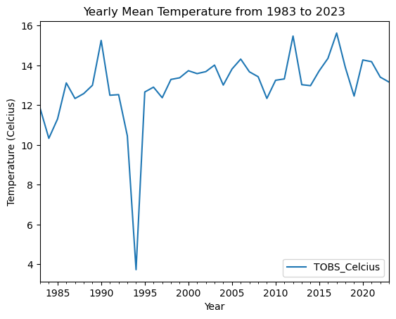
# Plot mean annual temperature values
climate_1983_2023_mean.plot(
    y='TOBS_Celcius',
    title='Yearly Mean Temperature from 1983 to 2023',
    xlabel='Year',
    ylabel='Temperature (Celcius)'
)
<Axes: title={'center': 'Yearly Mean Temperature from 1983 to 2023'}, xlabel='Year', ylabel='Temperature (Celcius)'>
Describe your plot
We like to use an approach called “Assertion-Evidence” for presenting scientific results. There’s a lot of video tutorials and example talks available on the Assertion-Evidence web page. The main thing you need to do now is to practice writing a message or headline rather than descriptions or topic sentences for the plot you just made (what they refer to as “visual evidence”).
For example, it would be tempting to write something like “A plot of maximum annual temperature in Boulder, Colorado over time (1983-2023)”. However, this doesn’t give the reader anything to look at, or explain why we made this particular plot (we know, you made this one because we told you to)
Some alternatives for different plots of Boulder temperature that are more of a starting point for a presentation or conversation are:
- Boulder, CO experienced cooler than average temperatures in 1995
- Temperatures in Bouler, CO appear to be on the rise over the past 40 years
- Maximum annual temperatures in Boulder, CO are becoming more variable over the previous 40 years
We could back up some of these claims with further analysis included later on, but we want to make sure that our audience has some guidance on what to look for in the plot.
1994 Was a Historically Cold Year for Boulder,CO 📰 🗞️ 📻
Looking at historical climate data by NOAA, mean temperatures were calculated from 1983 to 2023 at a Boulder weather station. After analysing the dataset, scientists perceived the year 1994 as having a dip of almost 10 degrees. Boulder hasn’t seen a dip this large since.

Image credit: https://www.craiyon.com/image/OAbZtyelSoS7FdGko6hvQg
THIS ISN’T THE END! 😄
Don’t forget to reproduce your analysis in a new location or time!
Image source: https://www.independent.co.uk/climate-change/news/by-the-left-quick-march-the-emperor-penguins-migration-1212420.html
Your turn: pick a new location and/or measurement to plot 🌏 📈
Below (or in a new notebook!), recreate the workflow you just did in a place that interests you OR with a different measurement. See the instructions above to adapt the URL that we created for Boulder, CO using the NCEI API. You will need to make your own new Markdown and Code cells below this one, or create a new notebook.
Congratulations, you’re almost done with this coding challenge 🤩 – now make sure that your code is reproducible

Image source: https://dfwurbanwildlife.com/2018/03/25/chris-jacksons-dfw-urban-wildlife/snow-geese-galore/
Your task
If you didn’t already, go back to the code you modified about and write more descriptive comments so the next person to use this code knows what it does.
Make sure to
RestartandRun allup at the top of your notebook. This will clear all your variables and make sure that your code runs in the correct order. It will also export your work in Markdown format, which you can put on your website.
BONUS: Create a shareable Markdown of your work
Below is some code that you can run that will save a Markdown file of your work that is easily shareable and can be uploaded to GitHub Pages. You can use it as a starting point for writing your portfolio post!
%%capture
%%bash
jupyter nbconvert *.ipynb --to markdown